Building GBDT Inference on Encrypted Data with CKKS

The Challenge: Privacy-Preserving Ensembles

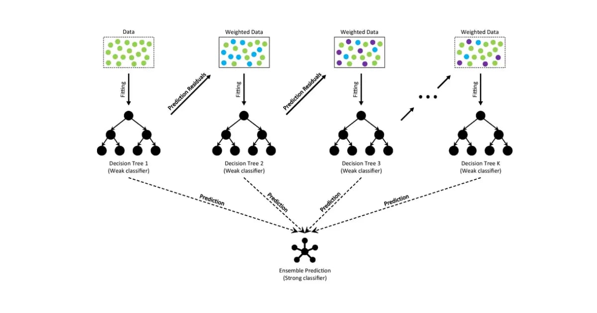
Gradient Boosting Decision Trees (GBDT) are a workhorse of modern machine learning, but deploying them in a “Machine Learning as a Service” (MLaaS) model creates a privacy deadlock: clients are unwilling to disclose sensitive features, and providers must protect their proprietary models.

Homomorphic Encryption (HE) offers a way out, allowing a service provider to compute on encrypted data. However, there is a persistent gap between academic HE papers and production-minded implementations. Papers tend to compress the hard parts—mapping branching logic to arithmetic, controlling multiplicative depth, and bridging ML stacks with HE runtimes—into a few sentences.

In this guide, we’ll walk through the architecture of building a GBDT inference engine on encrypted data using the CKKS (Cheon-Kim-Kim-Song) scheme, based on the foundational approach proposed by Xiao et al. (2019).

This is the first in a series of posts on privacy-preserving machine learning. You can find the reference implementation at github.com/chuckchen/ckks-gbdt.

Summary of Results

Before diving into the architecture, here is how the implementation performed compared to the plaintext baseline on held-out test slices:

Dataset	Metric	Plaintext (Baseline)	Encrypted (Reproduction)	Gap
Credit	Micro-F1	0.7344	0.7188	-0.0156
MNIST	Micro-F1	1.0000	0.8750*	-0.1250

*Note: MNIST encrypted result is from the HE-style surrogate (polynomialized approximation) used to verify the routing logic without the high computational cost of a full CKKS run on multiclass ensembles.

1. The Core Idea: Polynomialization

The central problem in HE is that it only supports addition and multiplication. In a standard GBDT, a split at an internal node $v$ is a discrete choice:

$$\text{Branch}(x_j, s_v) = \begin{cases} \text{left} & \text{if } x_j \le s_v \\ \text{right} &\; \text{otherwise} \end{cases}$$

To evaluate this under CKKS, we must transform this control flow into a continuous arithmetic circuit.

Approximating the Comparison

We first replace the discrete indicator with a “soft” routing variable $a_v$. Ideally, $a_v = \text{sign}(s_v - x_j)$, but since the sign function is non-continuous, we approximate it using a parameterized sigmoid function:

$$\sigma(x; t) = \frac{1}{1 + \exp(-t \cdot x)}$$

where $t$ is a steepness factor (typically 128). This gives us $a_v \approx \sigma(s_v - x_j; t)$, where $a_v \to 1$ if the condition is met and $a_v \to 0$ otherwise.

The Decision Tree Polynomial

Theorem 1 in the Xiao et al. paper guarantees that any decision tree $T$ can be uniquely represented as a polynomial $P(T)$. For a node $v$ with left child $T_L$ and right child $T_R$, the output is defined recursively:

$$P(T) = a_v \cdot P(T_L) + (1 - a_v) \cdot P(T_R)$$

By unrolling this recursion, the final score of a tree is the sum of contributions from every leaf $L$:

$$P(T) = \sum_{L \in \text{Leaves}} \text{Value}(L) \cdot \prod_{v \in \text{Path}(L)} \mathbf{c}_v$$

where the condition term $\mathbf{c}_v$ is $a_v$ if the path goes left at node $v$, and $(1 - a_v)$ if it goes right. This transformation turns the discrete tree into a sum-of-products circuit that CKKS can evaluate.

Why Chebyshev Polynomials?

To evaluate the sigmoid function homomorphically, we use a degree-24 Chebyshev polynomial. Unlike Taylor series, which are local approximations, Chebyshev polynomials minimize the maximum error ($L_\infty$ norm) over an entire interval (typically $[-1, 1]$). This ensures the approximation is stable even for values far from the threshold, preventing incorrect routing in deeper layers.

2. Optimizing for Scalability: $O(\log n)$ Depth

A naive recursive evaluation of a tree polynomial leads to a multiplicative depth that grows linearly with the tree’s depth. In FHE, multiplicative depth is our most expensive resource.

Xiao et al. demonstrate that we can reduce this to $O(\log n)$ using a Balanced Product Tree strategy. Instead of multiplying path terms sequentially:

$$(a_1 \cdot a_2) \cdot a_3 \dots \cdot a_d$$

We pair them up and perform parallel multiplications:

$$(a_1 \cdot a_2) \cdot (a_3 \cdot a_4) \dots$$

This strategy is what makes the circuit depth manageable, allowing us to support deeper ensembles without exhausting the CKKS modulus chain.

3. Systems Optimization: Vertical Packing

Efficiency in CKKS comes from SIMD (Single Instruction, Multiple Data) operations. Most ML implementations are row-oriented (one sample, all features). To build an efficient encrypted runtime, we must think “column-oriented”.

In Vertical Packing, we pack the same feature across many different samples into a single ciphertext.

• The Benefit: When a node splits on feature $j$, we only load one ciphertext ($ct_j$).
• The Scale: A single homomorphic operation now processes thousands of samples simultaneously (e.g., 8,192 slots).
• Decoupled Latency: Batch latency becomes almost entirely dependent on model complexity, rather than batch size (up to the slot limit).

4. Implementation Architecture

Building a production-minded HE system requires a clean boundary between the ML stack and the cryptographic circuit.

Layer 1: The Pre-processing Pipeline (Python)

We use lightgbm to train the model, then export it into a flat, library-agnostic contract (model.txt).

• Folding Shrinkage: We multiply the learning rate (shrinkage) directly into the leaf values at export time. This saves one encrypted multiplication and rescale step per tree—a critical optimization that often determines success in deep circuits.

Layer 2: The Homomorphic Runtime (C++)

Built on the original HEAAN library, the runtime loads the tree bundle and executes the $O(\log n)$ circuit using the Paterson-Stockmeyer algorithm to minimize non-scalar multiplications.

5. Performance and Error Bounds

Xiao et al. provided a critical theoretical bound for the absolute error $|e(G)|$:

$$|e(G)| \le \sum_{i=1}^n \left| \frac{\partial G}{\partial a_i} \right| \cdot \delta(a_i)$$

Because GBDT is an ensemble of many trees, the partial derivatives $\frac{\partial G}{\partial a_i}$ are generally small, helping the overall error remain bounded even as the number of features $n$ grows.

Debugging the Arithmetic Budget

The hardest bugs were not typical C++ bugs (like segfaults) but HE arithmetic failures. For example, a division by zero in _ntl_gdiv failure from NTL is often a symptom of modulus exhaustion. In FHE, “cryptographic budgeting” replaces “FLOP counting”—the fix rarely involves changing the logic; it involves resizing CKKS parameters or reordering the path-product tree to save a level of depth.

Closing Thought

The most satisfying part of building this system was watching the abstractions of the paper survive contact with real-world constraints—file formats, build systems, and modulus budgets. Bridging the gap between theory and implementation is where the most useful engineering insights are found.

In the next post, we will explore the MNIST Challenge: scaling this architecture to multi-class ensembles and handling the exponential increase in multiplicative depth requirements.