Number Theoretic Transform (NTT): Math, Example & Python

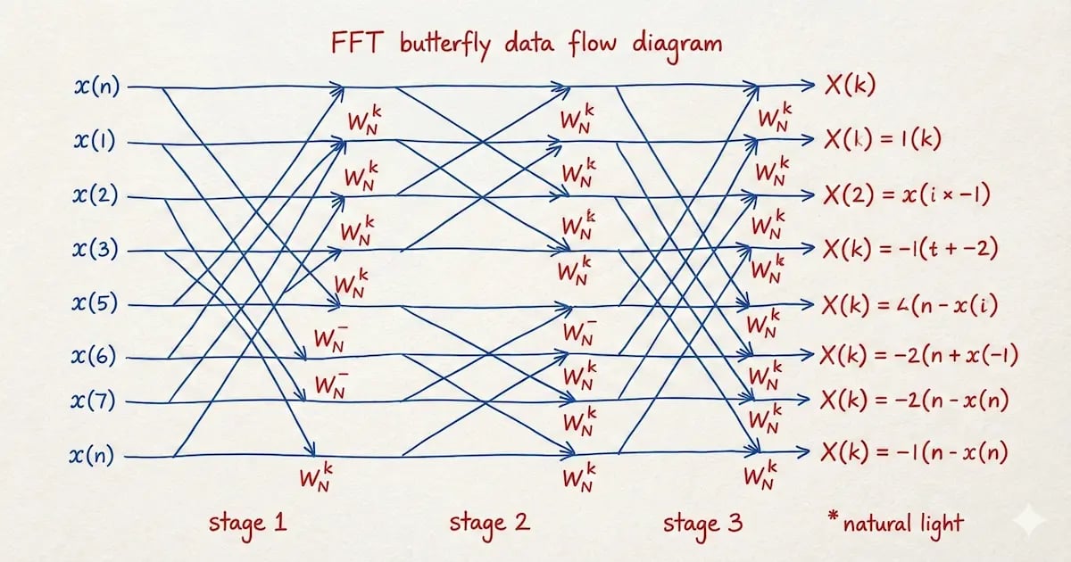
The Number Theoretic Transform (NTT) is a discrete Fourier transform over a finite field. It converts polynomial coefficients into values at roots of unity, so multiplication can be performed point by point and reversed with an inverse NTT. All arithmetic is exact modulo the chosen prime.

This guide explains the NTT and inverse formulas, works through a multiplication modulo 17, and provides Python code you can run. You only need basic polynomial multiplication and modular arithmetic.

NTT vs FFT

Both can accelerate polynomial multiplication to $O(n \log n)$. NTT is useful when exact modular coefficients are needed; it does not by itself encrypt data or guarantee cryptographic security. FFT-based integer multiplication can also be exact when rounding error is bounded carefully.

The Problem with FFT in Cryptography

A complex FFT evaluates a polynomial at complex roots of unity. In a floating-point implementation, rounding error must be controlled before recovering integer coefficients. A finite-field NTT avoids that rounding step for modular arithmetic, provided its parameters meet the conditions below.

Enter NTT: The Integer-Based Solution

The Number Theoretic Transform (NTT) solves the precision problem by swapping the world of complex numbers for the world of modular arithmetic. Instead of operating on an infinite field of complex numbers, the NTT operates on a finite field of integers modulo a prime number $p$.

This has two key advantages:

1. No Floating-Point Errors: All calculations are done with integers, ensuring perfect precision.
2. Efficiency: The calculations remain incredibly fast, inheriting the $O(n \log n)$ speed of the FFT algorithm.

The magic ingredient that makes this work is finding an integer equivalent of the “primitive root of unity” used in the FFT. In the NTT, we find a special integer $\omega$ (omega) in our finite field that behaves just like its complex counterpart, allowing us to perform the transform and its inverse.

Choosing the length, modulus, and root

For the radix-2 implementation below:

• Choose a power-of-two length $n$. For input lengths $r$ and $s$, use $n \ge r+s-1$ and pad both coefficient vectors with zeros.
• Choose a prime $p$ with $n \mid (p-1)$, so the field contains a primitive $n$-th root of unity.
• Choose $\omega$ with exact order $n$. For power-of-two $n>1$, check $\omega^n=1$ and $\omega^{n/2}\ne1$ modulo $p$. Checking only $\omega^n=1$ would incorrectly accept $\omega=1$.
• If $g$ is a generator of the nonzero field elements, $\omega=g^{(p-1)/n}\bmod p$ is one way to obtain the root.

Linear vs cyclic convolution

An $n$-point NTT computes multiplication modulo $x^n-1$: coefficients beyond degree $n-1$ wrap around. This is cyclic convolution. Padding to at least $r+s-1$ prevents wraparound and gives the ordinary linear convolution, with coefficients still reduced modulo $p$.

Recovering unrestricted integer coefficients needs a sufficiently large modulus (or several primes and the Chinese Remainder Theorem). For signed coefficients bounded in magnitude by $B$, a modulus greater than $2B$ permits signed reconstruction. The small example below needs no reconstruction because every result coefficient lies between 0 and 16.

Multiplication modulo $x^n+1$ is negacyclic convolution and requires a different construction; the code below does not implement it.

A Step-by-Step Walkthrough

Let’s walk through a concrete example of multiplying two polynomials using the NTT. We will calculate the product of $A(x) = 2x + 1$ and $B(x) = 3x + 4$.

1. Setup

We need to choose our parameters:

• Modulus ($p$): 17. We will work in the field of integers modulo 17.
• Transform Size ($n$): 4. The product of two degree-1 polynomials has degree 2. To avoid aliasing, $n$ must be a power of 2 greater than 2. We pad our coefficient vectors with zeros to length 4.
• Root of Unity ($\omega$): 13. We need an element $\omega$ such that $\omega^4 \equiv 1 \pmod{17}$. $13^1 = 13$, $13^2 \equiv 16 \equiv -1$, $13^3 \equiv 4$, $13^4 \equiv 1$.
• Inverse of $n$ ($n^{-1}$): 13. Since $4 \times 13 = 52 = 3 \times 17 + 1$, the modular inverse of 4 is 13.

Our input vectors are:

• $a = [1, 2, 0, 0]$ (representing $1 + 2x$)
• $b = [4, 3, 0, 0]$ (representing $4 + 3x$)

2. Forward NTT

We transform vector $a$ into point-value form $A$ using the formula $A_k = \sum_{j=0}^{n-1} a_j \omega^{jk} \pmod{17}$.

• $A_0 = 1 + 2(13)^0 + 0 + 0 = 3$

• $A_1 = 1 + 2(13)^1 = 1 + 26 = 27 \equiv \mathbf{10}$

• $A_2 = 1 + 2(13)^2 = 1 + 2(16) = 33 \equiv \mathbf{16}$

• $A_3 = 1 + 2(13)^3 = 1 + 2(4) = 9 \equiv \mathbf{9}$

  $A = [3, 10, 16, 9]$

Similarly for vector $b$:

• $B_0 = 4 + 3(13)^0 = 7$

• $B_1 = 4 + 3(13)^1 = 4 + 39 = 43 \equiv \mathbf{9}$

• $B_2 = 4 + 3(13)^2 = 4 + 3(16) = 52 \equiv \mathbf{1}$

• $B_3 = 4 + 3(13)^3 = 4 + 3(4) = 16 \equiv \mathbf{16}$

  $B = [7, 9, 1, 16]$

3. Point-wise Multiplication

We multiply the transformed vectors element-by-element modulo 17 to get $C$.

• $C_0 = 3 \times 7 = 21 \equiv \mathbf{4}$

• $C_1 = 10 \times 9 = 90 \equiv \mathbf{5}$

• $C_2 = 16 \times 1 = \mathbf{16}$

• $C_3 = 9 \times 16 = 144 \equiv \mathbf{8}$

  $C = [4, 5, 16, 8]$

4. Inverse NTT (INTT)

Now we transform $C$ back to coefficients using the inverse formula. We use $\omega^{-1} = 4$ (since $13 \times 4 = 52 \equiv 1$) and multiply the final result by $n^{-1} = 13$.

First, let’s compute the summation $S_j = \sum_{k=0}^{n-1} C_k (\omega^{-1})^{jk} \pmod{17}$:

• $S_0 = 4(1) + 5(1) + 16(1) + 8(1) = 33 \equiv 16$
• $S_1 = 4(1) + 5(4) + 16(16) + 8(13) \equiv 4 + 3 + 1 + 2 = 10$
• $S_2 = 4(1) + 5(16) + 16(256) + 8(169) \equiv 4 + 12 + 16 + 9 = 41 \equiv 7$
• $S_3 = 4(1) + 5(13) + 16(169) + 8(2197) \equiv 4 + 14 + 1 + 15 = 34 \equiv 0$

Finally, multiply by $n^{-1} = 13$:

• $c_0 = 16 \times 13 = 208 \equiv \mathbf{4}$
• $c_1 = 10 \times 13 = 130 \equiv \mathbf{11}$
• $c_2 = 7 \times 13 = 91 \equiv \mathbf{6}$
• $c_3 = 0 \times 13 = \mathbf{0}$

The result is $c = [4, 11, 6, 0]$, which corresponds to the polynomial $6x^2 + 11x + 4$. Matches the standard multiplication: $(2x+1)(3x+4) = 6x^2 + 11x + 4$.

The NTT and INTT Algorithms

For those who want a deeper look, let’s examine the forward and inverse transforms. The NTT takes a polynomial’s coefficient vector $a$ and transforms it into a point-value representation $A$. The INTT reverses this process.

The forward NTT is defined as: $A_k = \sum_{j=0}^{n-1} a_j \omega^{jk} \pmod{N}$

And the Inverse NTT is defined as: $a_j = (n^{-1}) \sum_{k=0}^{n-1} A_k \omega^{-jk} \pmod{N}$

Where:

• $a$ is the input vector of coefficients.
• $A$ is the transformed output vector.
• $N$ is the prime modulus.
• $n$ is the transform size (a power of 2 for this implementation).
• $\omega$ is a primitive $n$-th root of unity modulo $N$.
• $n^{-1}$ is the modular multiplicative inverse of $n$ modulo $N$.

Why does the inverse NTT multiply by $n^{-1}$?

For a primitive $n$-th root, $\sum_{k=0}^{n-1}\omega^{(j-\ell)k}$ is $n$ when $j=\ell$, and zero otherwise. Applying the inverse root therefore recovers $n$ times each original coefficient. Multiplying by the modular inverse of $n$ removes that factor. In the example, $n^{-1}=13$ because $4\cdot13\equiv1\pmod{17}$.

Here is an illustrative Python implementation of the NTT, which is analogous to the Cooley-Tukey FFT algorithm.

def ntt(a, N, w, n):
    """Radix-2 NTT; N must be a prime supplied by the caller."""
    if n < 1 or n & (n - 1) or len(a) != n:
        raise ValueError("Use a power-of-two length matching the input")
    if N < 2 or (N - 1) % n:
        raise ValueError("The prime modulus must satisfy n | (N - 1)")
    if pow(w, n, N) != 1 or (n > 1 and pow(w, n // 2, N) == 1):
        raise ValueError("The root must have exact order n")
    # 1. Bit-reversal permutation
    A = [value % N for value in a]
    for i in range(n):
        rev_i = int(f'{i:0{n.bit_length()-1}b}'[::-1], 2)
        if i < rev_i:
            A[i], A[rev_i] = A[rev_i], A[i]
 
    # 2. Butterfly operations
    s = 1
    while (m := 2**s) <= n:
        w_m = pow(w, n // m, N)
        for k in range(0, n, m):
            w_pow = 1
            for j in range(m // 2):
                u = A[k + j]
                t = (A[k + j + m // 2] * w_pow) % N
                A[k + j] = (u + t) % N
                A[k + j + m // 2] = (u - t + N) % N
                w_pow = (w_pow * w_m) % N
        s += 1
    return A

And here is the Python code for the Inverse NTT. Notice it’s nearly identical, just using the inverse root of unity and scaling the final result.

def intt(A, N, w_inv, n):
    """Inverse Number Theoretic Transform"""
    # The INTT algorithm is the same as NTT, just with the inverse root
    a = ntt(A, N, w_inv, n)
 
    # Scale the result by n_inv
    n_inv = pow(n, N - 2, N)
    for i in range(n):
        a[i] = (a[i] * n_inv) % N
    return a

The bit-reversal step is a pre-processing permutation that reorders the input array to be in the correct order for the iterative butterfly operations that follow. This reordering is what allows the algorithm to be so efficient.

Run the complete Python example

Run the two functions above followed by this block with Python 3.8 or later. Coefficients are ordered from constant term upwards. This is an educational implementation; it does not implement constant-time cryptographic operations.

p, n, w = 17, 4, 13
a = [1, 2, 0, 0]
b = [4, 3, 0, 0]
A = ntt(a, p, w, n)
B = ntt(b, p, w, n)
C = [x * y % p for x, y in zip(A, B)]
c = intt(C, p, pow(w, -1, p), n)
 
assert intt(A, p, pow(w, -1, p), n) == a
assert c == [4, 11, 6, 0]
print("NTT(a):", A)
print("NTT(b):", B)
print("Product coefficients:", c)

NTT(a): [3, 10, 16, 9]
NTT(b): [7, 9, 1, 16]
Product coefficients: [4, 11, 6, 0]

Beyond the Standard NTT: Variants and Cousins

While the standard Number Theoretic Transform is the workhorse of modern cryptography, it is part of a larger family of transforms, each optimized for specific constraints or mathematical structures.

• Discrete Fourier Transform (DFT): The grandfather of them all. While NTT operates on finite fields of integers, DFT operates on the field of complex numbers. The Fast Fourier Transform (FFT) is simply an efficient algorithm to compute the DFT.
• Discrete Cosine Transform (DCT): A close relative of the DFT that uses only real numbers and cosine functions. It is best known for its “energy compaction” properties in signal processing (powering JPEG and MP3), but number-theoretic variants also exist for specialized integer arithmetic applications.
• Discrete Galois Transform (DGT): A specialized variant that operates over Galois extensions of finite fields (e.g., Gaussian integers modulo $p$). It effectively packs more information into each element, potentially halving the transform length required for a given polynomial degree. This is particularly relevant in optimizing post-quantum schemes like Kyber.
• Discrete Weighted Transform (DWT): A variation that applies weight factors to the input and output vectors. This is often used to perform “negacyclic” convolutions (common in lattice cryptography) or to compute linear convolutions without the full zero-padding overhead required by the standard cyclic convolution.
• Walsh-Hadamard Transform (WHT): A simplified transform that uses only additions and subtractions (no multiplications). While less powerful for general convolution than NTT/FFT, its speed makes it valuable in quantum algorithms, error-correcting codes, and specific cryptographic booleans.
• Irrational Base Discrete Weighted Transform (IBDWT): A flavor of DWT used in computations involving massive numbers (such as the Great Internet Mersenne Prime Search). It allows for efficient multiplication using floating-point hardware while maintaining exact integer results through careful error analysis.

Quick Comparison

Why is NTT a Game-Changer for Cryptography?

The primary application of NTT in cryptography is to perform fast polynomial multiplication. Many modern cryptographic schemes, especially those based on lattices, are built on operations involving very large polynomials.

Doing this multiplication naively would be too slow to be practical. The NTT provides a massive speedup, making these advanced cryptographic schemes feasible.

NIST’s ML-KEM standard (FIPS 203), derived from CRYSTALS-Kyber, specifies a key-encapsulation mechanism. ML-DSA (FIPS 204), derived from CRYSTALS-Dilithium, specifies digital signatures. Their NTT constructions and parameters are scheme-specific; the teaching implementation above is not a replacement for either standard.

For the surrounding algebra, see the cryptography equations guide. For how polynomial arithmetic fits into encrypted computation, continue with BGV, BFV, and CKKS.

Conclusion

The Number Theoretic Transform is a cornerstone of modern cryptography, providing the speed and precision necessary to build the secure systems of tomorrow. While it operates deep under the hood, this elegant mathematical tool is what makes it possible to create cryptographic systems that are not only safe from today’s computers but also from the quantum threats of the future. It’s a perfect example of how abstract mathematics finds powerful, practical applications in securing our digital world.